A Gentle Introduction to Algorithm Complexity Analysis
Dionysis "dionyziz" Zindros <dionyziz@gmail.com>- English
- Ελληνικά
- македонски
- Español
- Nederlands
- עברית
- Português
- srpskohrvatski
- Українська
- Русский
- Help translate
Introduction
A lot of programmers that make some of the coolest and most useful software today, such as many of the stuff we see on the Internet or use daily, don't have a theoretical computer science background. They're still pretty awesome and creative programmers and we thank them for what they build.
However, theoretical computer science has its uses and applications and can turn out to be quite practical. In this article, targeted at programmers who know their art but who don't have any theoretical computer science background, I will present one of the most pragmatic tools of computer science: Big O notation and algorithm complexity analysis. As someone who has worked both in a computer science academic setting and in building production-level software in the industry, this is the tool I have found to be one of the truly useful ones in practice, so I hope after reading this article you can apply it in your own code to make it better. After reading this post, you should be able to understand all the common terms computer scientists use such as "big O", "asymptotic behavior" and "worst-case analysis".
This text is also targeted at the junior high school and high school students from Greece or anywhere else internationally competing in the International Olympiad in Informatics, an algorithms competition for students, or other similar competitions. As such, it does not have any mathematical prerequisites and will give you the background you need in order to continue studying algorithms with a firmer understanding of the theory behind them. As someone who used to compete in these student competitions, I highly advise you to read through this whole introductory material and try to fully understand it, because it will be necessary as you study algorithms and learn more advanced techniques.
I believe this text will be helpful for industry programmers who don't have too much experience with theoretical computer science (it is a fact that some of the most inspiring software engineers never went to college). But because it's also for students, it may at times sound a little bit like a textbook. In addition, some of the topics in this text may seem too obvious to you; for example, you may have seen them during your high school years. If you feel you understand them, you can skip them. Other sections go into a bit more depth and become slightly theoretical, as the students competing in this competition need to know more about theoretical algorithms than the average practitioner. But these things are still good to know and not tremendously hard to follow, so it's likely well worth your time. As the original text was targeted at high school students, no mathematical background is required, so anyone with some programming experience (i.e. if you know what recursion is) will be able to follow through without any problem.
Throughout this article, you will find various pointers that link you to interesting material often outside the scope of the topic under discussion. If you're an industry programmer, it's likely that you're familiar with most of these concepts. If you're a junior student participating in competitions, following those links will give you clues about other areas of computer science or software engineering that you may not have yet explored which you can look at to broaden your interests.
Big O notation and algorithm complexity analysis is something a lot of industry programmers and junior students alike find hard to understand, fear, or avoid altogether as useless. But it's not as hard or as theoretical as it may seem at first. Algorithm complexity is just a way to formally measure how fast a program or algorithm runs, so it really is quite pragmatic. Let's start by motivating the topic a little bit.
Motivation
We already know there are tools to measure how fast a program runs. There are programs called profilers which measure running time in milliseconds and can help us optimize our code by spotting bottlenecks. While this is a useful tool, it isn't really relevant to algorithm complexity. Algorithm complexity is something designed to compare two algorithms at the idea level — ignoring low-level details such as the implementation programming language, the hardware the algorithm runs on, or the instruction set of the given CPU. We want to compare algorithms in terms of just what they are: Ideas of how something is computed. Counting milliseconds won't help us in that. It's quite possible that a bad algorithm written in a low-level programming language such as assembly runs much quicker than a good algorithm written in a high-level programming language such as Python or Ruby. So it's time to define what a "better algorithm" really is.
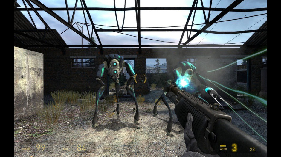
As algorithms are programs that perform just a computation, and not other things computers often do such as networking tasks or user input and output, complexity analysis allows us to measure how fast a program is when it performs computations. Examples of operations that are purely computational include numerical floating-point operations such as addition and multiplication; searching within a database that fits in RAM for a given value; determining the path an artificial-intelligence character will walk through in a video game so that they only have to walk a short distance within their virtual world (see Figure 1); or running a regular expression pattern match on a string. Clearly, computation is ubiquitous in computer programs.
Complexity analysis is also a tool that allows us to explain how an algorithm behaves as the input grows larger. If we feed it a different input, how will the algorithm behave? If our algorithm takes 1 second to run for an input of size 1000, how will it behave if I double the input size? Will it run just as fast, half as fast, or four times slower? In practical programming, this is important as it allows us to predict how our algorithm will behave when the input data becomes larger. For example, if we've made an algorithm for a web application that works well with 1000 users and measure its running time, using algorithm complexity analysis we can have a pretty good idea of what will happen once we get 2000 users instead. For algorithmic competitions, complexity analysis gives us insight about how long our code will run for the largest testcases that are used to test our program's correctness. So if we've measured our program's behavior for a small input, we can get a good idea of how it will behave for larger inputs. Let's start by a simple example: Finding the maximum element in an array.
Counting instructions
In this article, I'll use various programming languages for the examples. However, don't despair if you don't know a particular programming language. Since you know programming, you should be able to read the examples without any problem even if you aren't familiar with the programming language of choice, as they will be simple and I won't use any esoteric language features. If you're a student competing in algorithms competitions, you most likely work with C++, so you should have no problem following through. In that case I recommend working on the exercises using C++ for practice.
The maximum element in an array can be looked up using a simple piece of code such as this piece of Javascript code. Given an input array A of size n:
            var M = A[ 0 ];

            for ( var i = 0; i < n; ++i ) {
                if ( A[ i ] >= M ) {
                    M = A[ i ];
                }
            }
Now, the first thing we'll do is count how many fundamental instructions this piece of code executes. We will only do this once and it won't be necessary as we develop our theory, so bear with me for a few moments as we do this. As we analyze this piece of code, we want to break it up into simple instructions; things that can be executed by the CPU directly - or close to that. We'll assume our processor can execute the following operations as one instruction each:
- Assigning a value to a variable
- Looking up the value of a particular element in an array
- Comparing two values
- Incrementing a value
- Basic arithmetic operations such as addition and multiplication
We'll assume branching (the choice between if and else parts of code after the if condition has been evaluated) occurs instantly and won't count these instructions. In the above code, the first line of code is:
var M = A[ 0 ];
This requires 2 instructions: One for looking up A[ 0 ] and one for assigning the value to M (we're assuming that n is always at least 1). These two instructions are always required by the algorithm, regardless of the value of n. The for loop initialization code also has to always run. This gives us two more instructions; an assignment and a comparison:
            i = 0;
            i < n;
These will run before the first for loop iteration. After each for loop iteration, we need two more instructions to run, an increment of i and a comparison to check if we'll stay in the loop:
            ++i;
            i < n;
So, if we ignore the loop body, the number of instructions this algorithm needs is 4 + 2n. That is, 4 instructions at the beginning of the for loop and 2 instructions at the end of each iteration of which we have n. We can now define a mathematical function f( n ) that, given an n, gives us the number of instructions the algorithm needs. For an empty for body, we have f( n ) = 4 + 2n.
Worst-case analysis
Now, looking at the for body, we have an array lookup operation and a comparison that happen always:
if ( A[ i ] >= M ) { ...
That's two instructions right there. But the if body may run or may not run, depending on what the array values actually are. If it happens to be so that A[ i ] >= M, then we'll run these two additional instructions — an array lookup and an assignment:
M = A[ i ]
But now we can't define an f( n ) as easily, because our number of instructions doesn't depend solely on n but also on our input. For example, for A = [ 1, 2, 3, 4 ] the algorithm will need more instructions than for A = [ 4, 3, 2, 1 ]. When analyzing algorithms, we often consider the worst-case scenario. What's the worst that can happen for our algorithm? When does our algorithm need the most instructions to complete? In this case, it is when we have an array in increasing order such as A = [ 1, 2, 3, 4 ]. In that case, M needs to be replaced every single time and so that yields the most instructions. Computer scientists have a fancy name for that and they call it worst-case analysis; that's nothing more than just considering the case when we're the most unlucky. So, in the worst case, we have 4 instructions to run within the for body, so we have f( n ) = 4 + 2n + 4n = 6n + 4. This function f, given a problem size n, gives us the number of instructions that would be needed in the worst-case.
Asymptotic behavior
Given such a function, we have a pretty good idea of how fast an algorithm is. However, as I promised, we won't be needing to go through the tedious task of counting instructions in our program. Besides, the number of actual CPU instructions needed for each programming language statement depends on the compiler of our programming language and on the available CPU instruction set (i.e. whether it's an AMD or an Intel Pentium on your PC, or a MIPS processor on your Playstation 2) and we said we'd be ignoring that. We'll now run our "f" function through a "filter" which will help us get rid of those minor details that computer scientists prefer to ignore.
In our function, 6n + 4, we have two terms: 6n and 4. In complexity analysis we only care about what happens to the instruction-counting function as the program input (n) grows large. This really goes along with the previous ideas of "worst-case scenario" behavior: We're interested in how our algorithm behaves when treated badly; when it's challenged to do something hard. Notice that this is really useful when comparing algorithms. If an algorithm beats another algorithm for a large input, it's most probably true that the faster algorithm remains faster when given an easier, smaller input. From the terms that we are considering, we'll drop all the terms that grow slowly and only keep the ones that grow fast as n becomes larger. Clearly 4 remains a 4 as n grows larger, but 6n grows larger and larger, so it tends to matter more and more for larger problems. Therefore, the first thing we will do is drop the 4 and keep the function as f( n ) = 6n.
This makes sense if you think about it, as the 4 is simply an "initialization constant". Different programming languages may require a different time to set up. For example, Java needs some time to initialize its virtual machine. Since we're ignoring programming language differences, it only makes sense to ignore this value.
The second thing we'll ignore is the constant multiplier in front of n, and so our function will become f( n ) = n. As you can see this simplifies things quite a lot. Again, it makes some sense to drop this multiplicative constant if we think about how different programming languages compile. The "array lookup" statement in one language may compile to different instructions in different programming languages. For example, in C, doing A[ i ] does not include a check that i is within the declared array size, while in Pascal it does. So, the following Pascal code:
M := A[ i ]
Is the equivalent of the following in C:
            if ( i >= 0 && i < n ) {
                M = A[ i ];
            }
So it's reasonable to expect that different programming languages will yield different factors when we count their instructions. In our example in which we are using a dumb compiler for Pascal that is oblivious of possible optimizations, Pascal requires 3 instructions for each array access instead of the 1 instruction C requires. Dropping this factor goes along the lines of ignoring the differences between particular programming languages and compilers and only analyzing the idea of the algorithm itself.
This filter of "dropping all factors" and of "keeping the largest growing term" as described above is what we call asymptotic behavior. So the asymptotic behavior of f( n ) = 2n + 8 is described by the function f( n ) = n. Mathematically speaking, what we're saying here is that we're interested in the limit of function f as n tends to infinity; but if you don't understand what that phrase formally means, don't worry, because this is all you need to know. (On a side note, in a strict mathematical setting, we would not be able to drop the constants in the limit; but for computer science purposes, we want to do that for the reasons described above.) Let's work a couple of examples to familiarize ourselves with the concept.
Let us find the asymptotic behavior of the following example functions by dropping the constant factors and by keeping the terms that grow the fastest.
f( n ) = 5n + 12 gives f( n ) = n.
By using the exact same reasoning as above.
f( n ) = 109 gives f( n ) = 1.
We're dropping the multiplier 109 * 1, but we still have to put a 1 here to indicate that this function has a non-zero value.
f( n ) = n2 + 3n + 112 gives f( n ) = n2
Here, n2 grows larger than 3n for sufficiently large n, so we're keeping that.
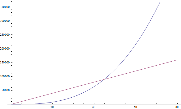
f( n ) = n3 + 1999n + 1337 gives f( n ) = n3
Even though the factor in front of n is quite large, we can still find a large enough n so that n3 is bigger than 1999n. As we're interested in the behavior for very large values of n, we only keep n3 (See Figure 2).
f( n ) = n +
 gives f( n ) = n
This is so because n grows faster than
as we increase n.
You can try out the following examples on your own:
Exercise 1
- f( n ) = n6 + 3n
- f( n ) = 2n + 12
- f( n ) = 3n + 2n
- f( n ) = nn + n
(Write down your results; the solution is given below)
If you're having trouble with one of the above, plug in some large n and see which term is bigger. Pretty straightforward, huh?
Complexity
So what this is telling us is that since we can drop all these decorative constants, it's pretty easy to tell the asymptotic behavior of the instruction-counting function of a program. In fact, any program that doesn't have any loops will have f( n ) = 1, since the number of instructions it needs is just a constant (unless it uses recursion; see below). Any program with a single loop which goes from 1 to n will have f( n ) = n, since it will do a constant number of instructions before the loop, a constant number of instructions after the loop, and a constant number of instructions within the loop which all run n times.
This should now be much easier and less tedious than counting individual instructions, so let's take a look at a couple of examples to get familiar with this. The following PHP program checks to see if a particular value exists within an array A of size n:
            <?php
                $exists = false;
                for ( $i = 0; $i < n; ++$i ) {
                    if ( $A[ $i ] == $value ) {
                        $exists = true;
                        break;
                    }
                }
            ?>
This method of searching for a value within an array is called linear search. This is a reasonable name, as this program has f( n ) = n (we'll define exactly what "linear" means in the next section). You may notice that there's a "break" statement here that may make the program terminate sooner, even after a single iteration. But recall that we're interested in the worst-case scenario, which for this program is for the array A to not contain the value. So we still have f( n ) = n.
Exercise 2
Systematically analyze the number of instructions the above PHP program needs with respect to n in the worst-case to find f( n ), similarly to how we analyzed our first Javascript program. Then verify that, asymptotically, we have f( n ) = n.
Let's look at a Python program which adds two array elements together to produce a sum which it stores in another variable:
v = a[ 0 ] + a[ 1 ]
Here we have a constant number of instructions, so we have f( n ) = 1.
The following program in C++ checks to see if a vector (a fancy array) named A of size n contains the same two values anywhere within it:
            bool duplicate = false;
            for ( int i = 0; i < n; ++i ) {
                for ( int j = 0; j < n; ++j ) {
                    if ( i != j && A[ i ] == A[ j ] ) {
                        duplicate = true;
                        break;
                    }
                }
                if ( duplicate ) {
                    break;
                }
            }
As here we have two nested loops within each other, we'll have an asymptotic behavior described by f( n ) = n2.
Rule of thumb: Simple programs can be analyzed by counting the nested loops of the program. A single loop over n items yields f( n ) = n. A loop within a loop yields f( n ) = n2. A loop within a loop within a loop yields f( n ) = n3.
If we have a program that calls a function within a loop and we know the number of instructions the called function performs, it's easy to determine the number of instructions of the whole program. Indeed, let's take a look at this C example:
            int i;
            for ( i = 0; i < n; ++i ) {
                f( n );
            }
If we know that f( n ) is a function that performs exactly n instructions, we can then know that the number of instructions of the whole program is asymptotically n2, as the function is called exactly n times.
Rule of thumb: Given a series of for loops that are sequential, the slowest of them determines the asymptotic behavior of the program. Two nested loops followed by a single loop is asymptotically the same as the nested loops alone, because the nested loops dominate the simple loop.
Now, let's switch over to the fancy notation that computer scientists use. When we've figured out the exact such f asymptotically, we'll say that our program is Θ( f( n ) ). For example, the above programs are Θ( 1 ), Θ( n2 ) and Θ( n2 ) respectively. Θ( n ) is pronounced "theta of n". Sometimes we say that f( n ), the original function counting the instructions including the constants, is Θ( something ). For example, we may say that f( n ) = 2n is a function that is Θ( n ) — nothing new here. We can also write 2n ∈ Θ( n ), which is pronounced as "two n is theta of n". Don't get confused about this notation: All it's saying is that if we've counted the number of instructions a program needs and those are 2n, then the asymptotic behavior of our algorithm is described by n, which we found by dropping the constants. Given this notation, the following are some true mathematical statements:
- n6 + 3n ∈ Θ( n6 )
- 2n + 12 ∈ Θ( 2n )
- 3n + 2n ∈ Θ( 3n )
- nn + n ∈ Θ( nn )
By the way, if you solved Exercise 1 from above, these are exactly the answers you should have found.
We call this function, i.e. what we put within Θ( here ), the time complexity or just complexity of our algorithm. So an algorithm with Θ( n ) is of complexity n. We also have special names for Θ( 1 ), Θ( n ), Θ( n2 ) and Θ( log( n ) ) because they occur very often. We say that a Θ( 1 ) algorithm is a constant-time algorithm, Θ( n ) is linear, Θ( n2 ) is quadratic and Θ( log( n ) ) is logarithmic (don't worry if you don't know what logarithms are yet – we'll get to that in a minute).
Rule of thumb: Programs with a bigger Θ run slower than programs with a smaller Θ.
Big-O notation
Now, it's sometimes true that it will be hard to figure out exactly the behavior of an algorithm in this fashion as we did above, especially for more complex examples. However, we will be able to say that the behavior of our algorithm will never exceed a certain bound. This will make life easier for us, as we won't have to specify exactly how fast our algorithm runs, even when ignoring constants the way we did before. All we'll have to do is find a certain bound. This is explained easily with an example.
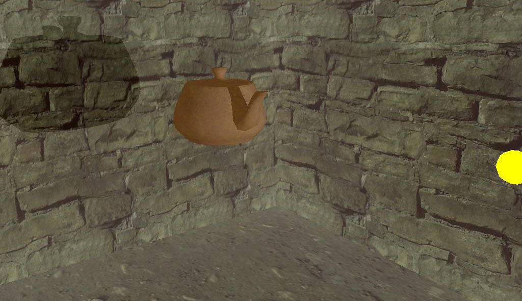
A famous problem computer scientists use for teaching algorithms is the sorting problem. In the sorting problem, an array A of size n is given (sounds familiar?) and we are asked to write a program that sorts this array. This problem is interesting because it is a pragmatic problem in real systems. For example, a file explorer needs to sort the files it displays by name so that the user can navigate them with ease. Or, as another example, a video game may need to sort the 3D objects displayed in the world based on their distance from the player's eye inside the virtual world in order to determine what is visible and what isn't, something called the Visibility Problem (see Figure 3). The objects that turn out to be closest to the player are those visible, while those that are further may get hidden by the objects in front of them. Sorting is also interesting because there are many algorithms to solve it, some of which are worse than others. It's also an easy problem to define and to explain. So let's write a piece of code that sorts an array.
Here is an inefficient way to implement sorting an array in Ruby. (Of course, Ruby supports sorting arrays using build-in functions which you should use instead, and which are certainly faster than what we'll see here. But this is here for illustration purposes.)
                b = []
                n.times do
                    m = a[ 0 ]
                    mi = 0
                    a.each_with_index do |element, i|
                        if element < m
                            m = element
                            mi = i
                        end
                    end
                    a.delete_at( mi )
                    b << m
                end
This method is called selection sort. It finds the minimum of our array (the array is denoted a above, while the minimum value is denoted m and mi is its index), puts it at the end of a new array (in our case b), and removes it from the original array. Then it finds the minimum between the remaining values of our original array, appends that to our new array so that it now contains two elements, and removes it from our original array. It continues this process until all items have been removed from the original and have been inserted into the new array, which means that the array has been sorted. In this example, we can see that we have two nested loops. The outer loop runs n times, and the inner loop runs once for each element of the array a. While the array a initially has n items, we remove one array item in each iteration. So the inner loop repeats n times during the first iteration of the outer loop, then n - 1 times, then n - 2 times and so forth, until the last iteration of the outer loop during which it only runs once.
It's a little harder to evaluate the complexity of this program, as we'd have to figure out the sum 1 + 2 + ... + (n - 1) + n. But we can for sure find an "upper bound" for it. That is, we can alter our program (you can do that in your mind, not in the actual code) to make it worse than it is and then find the complexity of that new program that we derived. If we can find the complexity of the worse program that we've constructed, then we know that our original program is at most that bad, or maybe better. That way, if we find out a pretty good complexity for our altered program, which is worse than our original, we can know that our original program will have a pretty good complexity too – either as good as our altered program or even better.
Let's now think of the way to edit this example program to make it easier to figure out its complexity. But let's keep in mind that we can only make it worse, i.e. make it take up more instructions, so that our estimate is meaningful for our original program. Clearly we can alter the inner loop of the program to always repeat exactly n times instead of a varying number of times. Some of these repetitions will be useless, but it will help us analyze the complexity of the resulting algorithm. If we make this simple change, then the new algorithm that we've constructed is clearly Θ( n2 ), because we have two nested loops where each repeats exactly n times. If that is so, we say that the original algorithm is O( n2 ). O( n2 ) is pronounced "big oh of n squared". What this says is that our program is asymptotically no worse than n2. It may even be better than that, or it may be the same as that. By the way, if our program is indeed Θ( n2 ), we can still say that it's O( n2 ). To help you realize that, imagine altering the original program in a way that doesn't change it much, but still makes it a little worse, such as adding a meaningless instruction at the beginning of the program. Doing this will alter the instruction-counting function by a simple constant, which is ignored when it comes to asymptotic behavior. So a program that is Θ( n2 ) is also O( n2 ).
But a program that is O( n2 ) may not be Θ( n2 ). For example, any program that is Θ( n ) is also O( n2 ) in addition to being O( n ). If we imagine the that a Θ( n ) program is a simple for loop that repeats n times, we can make it worse by wrapping it in another for loop which repeats n times as well, thus producing a program with f( n ) = n2. To generalize this, any program that is Θ( a ) is O( b ) when b is worse than a. Notice that our alteration to the program doesn't need to give us a program that is actually meaningful or equivalent to our original program. It only needs to perform more instructions than the original for a given n. All we're using it for is counting instructions, not actually solving our problem.
So, saying that our program is O( n2 ) is being on the safe side: We've analyzed our algorithm, and we've found that it's never worse than n2. But it could be that it's in fact n2. This gives us a good estimate of how fast our program runs. Let's go through a few examples to help you familiarize yourself with this new notation.
Exercise 3
Find out which of the following are true:
- A Θ( n ) algorithm is O( n )
- A Θ( n ) algorithm is O( n2 )
- A Θ( n2 ) algorithm is O( n3 )
- A Θ( n ) algorithm is O( 1 )
- A O( 1 ) algorithm is Θ( 1 )
- A O( n ) algorithm is Θ( 1 )
Solution
- We know that this is true as our original program was Θ( n ). We can achieve O( n ) without altering our program at all.
- As n2 is worse than n, this is true.
- As n3 is worse than n2, this is true.
- As 1 is not worse than n, this is false. If a program takes n instructions asymptotically (a linear number of instructions), we can't make it worse and have it take only 1 instruction asymptotically (a constant number of instructions).
- This is true as the two complexities are the same.
- This may or may not be true depending on the algorithm. In the general case it's false. If an algorithm is Θ( 1 ), then it certainly is O( n ). But if it's O( n ) then it may not be Θ( 1 ). For example, a Θ( n ) algorithm is O( n ) but not Θ( 1 ).
Exercise 4
Use an arithmetic progression sum to prove that the above program is not only O( n2 ) but also Θ( n2 ). If you don't know what an arithmetic progression is, look it up on Wikipedia – it's easy.
Because the O-complexity of an algorithm gives an upper bound for the actual complexity of an algorithm, while Θ gives the actual complexity of an algorithm, we sometimes say that the Θ gives us a tight bound. If we know that we've found a complexity bound that is not tight, we can also use a lower-case o to denote that. For example, if an algorithm is Θ( n ), then its tight complexity is n. Then this algorithm is both O( n ) and O( n2 ). As the algorithm is Θ( n ), the O( n ) bound is a tight one. But the O( n2 ) bound is not tight, and so we can write that the algorithm is o( n2 ), which is pronounced "small o of n squared" to illustrate that we know our bound is not tight. It's better if we can find tight bounds for our algorithms, as these give us more information about how our algorithm behaves, but it's not always easy to do.
Exercise 5
Determine which of the following bounds are tight bounds and which are not tight bounds. Check to see if any bounds may be wrong. Use o( notation ) to illustrate the bounds that are not tight.
- A Θ( n ) algorithm for which we found a O( n ) upper bound.
- A Θ( n2 ) algorithm for which we found a O( n3 ) upper bound.
- A Θ( 1 ) algorithm for which we found an O( n ) upper bound.
- A Θ( n ) algorithm for which we found an O( 1 ) upper bound.
- A Θ( n ) algorithm for which we found an O( 2n ) upper bound.
Solution
- In this case, the Θ complexity and the O complexity are the same, so the bound is tight.
- Here we see that the O complexity is of a larger scale than the Θ complexity so this bound is not tight. Indeed, a bound of O( n2 ) would be a tight one. So we can write that the algorithm is o( n3 ).
- Again we see that the O complexity is of a larger scale than the Θ complexity so we have a bound that isn't tight. A bound of O( 1 ) would be a tight one. So we can point out that the O( n ) bound is not tight by writing it as o( n ).
- We must have made a mistake in calculating this bound, as it's wrong. It's impossible for a Θ( n ) algorithm to have an upper bound of O( 1 ), as n is a larger complexity than 1. Remember that O gives an upper bound.
- This may seem like a bound that is not tight, but this is not actually true. This bound is in fact tight. Recall that the asymptotic behavior of 2n and n are the same, and that O and Θ are only concerned with asymptotic behavior. So we have that O( 2n ) = O( n ) and therefore this bound is tight as the complexity is the same as the Θ.
Rule of thumb: It's easier to figure out the O-complexity of an algorithm than its Θ-complexity.
You may be getting a little overwhelmed with all this new notation by now, but let's introduce just two more symbols before we move on to a few examples. These are easy now that you know Θ, O and o, and we won't use them much later in this article, but it's good to know them now that we're at it. In the example above, we modified our program to make it worse (i.e. taking more instructions and therefore more time) and created the O notation. O is meaningful because it tells us that our program will never be slower than a specific bound, and so it provides valuable information so that we can argue that our program is good enough. If we do the opposite and modify our program to make it better and find out the complexity of the resulting program, we use the notation Ω. Ω therefore gives us a complexity that we know our program won't be better than. This is useful if we want to prove that a program runs slowly or an algorithm is a bad one. This can be useful to argue that an algorithm is too slow to use in a particular case. For example, saying that an algorithm is Ω( n3 ) means that the algorithm isn't better than n3. It might be Θ( n3 ), as bad as Θ( n4 ) or even worse, but we know it's at least somewhat bad. So Ω gives us a lower bound for the complexity of our algorithm. Similarly to ο, we can write ω if we know that our bound isn't tight. For example, a Θ( n3 ) algorithm is ο( n4 ) and ω( n2 ). Ω( n ) is pronounced "big omega of n", while ω( n ) is pronounced "small omega of n".
Exercise 6
For the following Θ complexities write down a tight and a non-tight O bound, and a tight and non-tight Ω bound of your choice, providing they exist.
- Θ( 1 )
- Θ( )
- Θ( n )
- Θ( n2 )
- Θ( n3 )
Solution
This is a straight-forward application of the definitions above.
- The tight bounds will be O( 1 ) and Ω( 1 ). A non-tight O-bound would be O( n ). Recall that O gives us an upper bound. As n is of larger scale than 1 this is a non-tight bound and we can write it as o( n ) as well. But we cannot find a non-tight bound for Ω, as we can't get lower than 1 for these functions. So we'll have to do with the tight bound.
- The tight bounds will have to be the same as the Θ complexity, so they are O( ) and Ω( ) respectively. For non-tight bounds we can have O( n ), as n is larger than and so it is an upper bound for . As we know this is a non-tight upper bound, we can also write it as o( n ). For a lower bound that is not tight, we can simply use Ω( 1 ). As we know that this bound is not tight, we can also write it as ω( 1 ).
- The tight bounds are O( n ) and Ω( n ). Two non-tight bounds could be ω( 1 ) and o( n3 ). These are in fact pretty bad bounds, as they are far from the original complexities, but they are still valid using our definitions.
- The tight bounds are O( n2 ) and Ω( n2 ). For non-tight bounds we could again use ω( 1 ) and o( n3 ) as in our previous example.
- The tight bounds are O( n3 ) and Ω( n3 ) respectively. Two non-tight bounds could be ω( n2 ) and o( n3 ). Although these bounds are not tight, they're better than the ones we gave above.
The reason we use O and Ω instead of Θ even though O and Ω can also give tight bounds is that we may not be able to tell if a bound we've found is tight, or we may just not want to go through the process of scrutinizing it so much.
If you don't fully remember all the different symbols and their uses, don't worry about it too much right now. You can always come back and look them up. The most important symbols are O and Θ.
Also note that although Ω gives us a lower-bound behavior for our function (i.e. we've improved our program and made it perform less instructions) we're still referring to a "worst-case" analysis. This is because we're feeding our program the worst possible input for a given n and analyzing its behavior under this assumption.
The following table indicates the symbols we just introduced and their correspondence with the usual mathematical symbols of comparisons that we use for numbers. The reason we don't use the usual symbols here and use Greek letters instead is to point out that we're doing an asymptotic behavior comparison, not just a simple comparison.
| Asymptotic comparison operator | Numeric comparison operator |
|---|---|
| Our algorithm is o( something ) | A number is < something |
| Our algorithm is O( something ) | A number is ≤ something |
| Our algorithm is Θ( something ) | A number is = something |
| Our algorithm is Ω( something ) | A number is ≥ something |
| Our algorithm is ω( something ) | A number is > something |
Rule of thumb: While all the symbols O, o, Ω, ω and Θ are useful at times, O is the one used more commonly, as it's easier to determine than Θ and more practically useful than Ω.
Logarithms
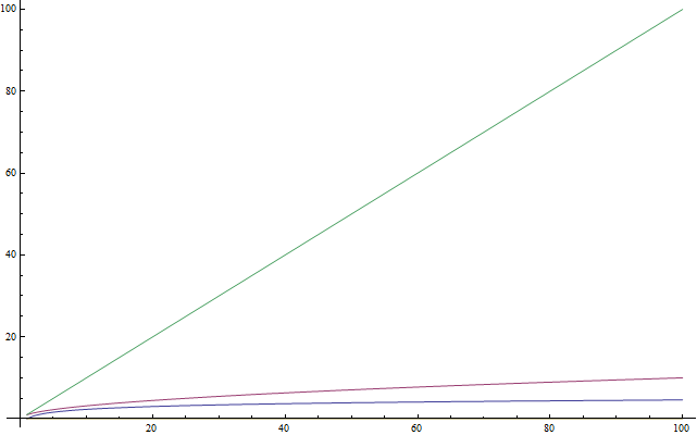
If you know what logarithms are, feel free to skip this section. As a lot of people are unfamiliar with logarithms, or just haven't used them much recently and don't remember them, this section is here as an introduction for them. This text is also for younger students that haven't seen logarithms at school yet. Logarithms are important because they occur a lot when analyzing complexity. A logarithm is an operation applied to a number that makes it quite smaller – much like a square root of a number. So if there's one thing you want to remember about logarithms is that they take a number and make it much smaller than the original (See Figure 4). Now, in the same way that square roots are the inverse operation of squaring something, logarithms are the inverse operation of exponentiating something. This isn't as hard as it sounds. It's better explained with an example. Consider the equation:
2x = 1024
We now wish to solve this equation for x. So we ask ourselves: What is the number to which we must raise the base 2 so that we get 1024? That number is 10. Indeed, we have 210 = 1024, which is easy to verify. Logarithms help us denote this problem using new notation. In this case, 10 is the logarithm of 1024 and we write this as log( 1024 ) and we read it as "the logarithm of 1024". Because we're using 2 as a base, these logarithms are called base 2 logarithms. There are logarithms in other bases, but we'll only use base 2 logarithms in this article. If you're a student competing in international competitions and you don't know about logarithms, I highly recommend that you practice your logarithms after completing this article. In computer science, base 2 logarithms are much more common than any other types of logarithms. This is because we often only have two different entities: 0 and 1. We also tend to cut down one big problem into halves, of which there are always two. So you only need to know about base-2 logarithms to continue with this article.
Exercise 7
Solve the equations below. Denote what logarithm you're finding in each case. Use only logarithms base 2.
- 2x = 64
- (22)x = 64
- 4x = 4
- 2x = 1
- 2x + 2x = 32
- (2x) * (2x) = 64
Solution
There is nothing more to this than applying the ideas defined above.
- By trial and error we can find that x = 6 and so log( 64 ) = 6.
- Here we notice that (22)x, by the properties of exponents, can be written as 22x. So we have that 2x = 6 because log( 64 ) = 6 from the previous result and therefore x = 3.
- Using our knowledge from the previous equation, we can write 4 as 22 and so our equation becomes (22)x = 4 which is the same as 22x = 4. Then we notice that log( 4 ) = 2 because 22 = 4 and therefore we have that 2x = 2. So x = 1. This is readily observed from the original equation, as using an exponent of 1 yields the base as a result.
- Recall that an exponent of 0 yields a result of 1. So we have log( 1 ) = 0 as 20 = 1, and so x = 0.
- Here we have a sum and so we can't take the logarithm directly. However we notice that 2x + 2x is the same as 2 * (2x). So we've multiplied in yet another two, and therefore this is the same as 2x + 1 and now all we have to do is solve the equation 2x + 1 = 32. We find that log( 32 ) = 5 and so x + 1 = 5 and therefore x = 4.
- We're multiplying together two powers of 2, and so we can join them by noticing that (2x) * (2x) is the same as 22x. Then all we need to do is to solve the equation 22x = 64 which we already solved above and so x = 3.
Rule of thumb: For competition algorithms implemented in C++, once you've analyzed your complexity, you can get a rough estimate of how fast your program will run by expecting it to perform about 1,000,000 operations per second, where the operations you count are given by the asymptotic behavior function describing your algorithm. For example, a Θ( n ) algorithm takes about a second to process the input for n = 1,000,000.
Recursive complexity
Let's now take a look at a recursive function. A recursive function is a function that calls itself. Can we analyze its complexity? The following function, written in Python, evaluates the factorial of a given number. The factorial of a positive integer number is found by multiplying it with all the previous positive integers together. For example, the factorial of 5 is 5 * 4 * 3 * 2 * 1. We denote that "5!" and pronounce it "five factorial" (some people prefer to pronounce it by screaming it out aloud like "FIVE!!!")
                def factorial( n ):
                    if n == 1:
                        return 1
                    return n * factorial( n - 1 )
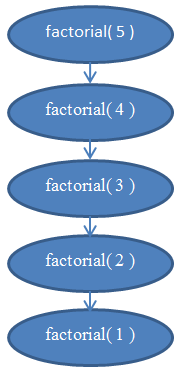
Let us analyze the complexity of this function. This function doesn't have any loops in it, but its complexity isn't constant either. What we need to do to find out its complexity is again to go about counting instructions. Clearly, if we pass some n to this function, it will execute itself n times. If you're unsure about that, run it "by hand" now for n = 5 to validate that it actually works. For example, for n = 5, it will execute 5 times, as it will keep decreasing n by 1 in each call. We can see therefore that this function is then Θ( n ).
If you're unsure about this fact, remember that you can always find the exact complexity by counting instructions. If you wish, you can now try to count the actual instructions performed by this function to find a function f( n ) and see that it's indeed linear (recall that linear means Θ( n )).
See Figure 5 for a diagram to help you understand the recursions performed when factorial( 5 ) is called.
This should clear up why this function is of linear complexity.
Logarithmic complexity
One famous problem in computer science is that of searching for a value within an array. We solved this problem earlier for the general case. This problem becomes interesting if we have an array which is sorted and we want to find a given value within it. One method to do that is called binary search. We look at the middle element of our array: If we find it there, we're done. Otherwise, if the value we find there is bigger than the value we're looking for, we know that our element will be on the left part of the array. Otherwise, we know it'll be on the right part of the array. We can keep cutting these smaller arrays in halves until we have a single element to look at. Here's the method using pseudocode:
                def binarySearch( A, n, value ):
                    if n = 1:
                        if A[ 0 ] = value:
                            return true
                        else:
                            return false
                    if value < A[ n / 2 ]:
                        return binarySearch( A[ 0...( n / 2 - 1 ) ], n / 2 - 1, value )
                    else if value > A[ n / 2 ]:
                        return binarySearch( A[ ( n / 2 + 1 )...n ], n / 2 - 1, value )
                    else:
                        return true
This pseudocode is a simplification of the actual implementation. In practice, this method is easier described than implemented, as the programmer needs to take care of some implementation issues. There are off-by-one errors and the division by 2 may not always produce an integer value and so it's necessary to floor() or ceil() the value. But we can assume for our purposes that it will always succeed, and we'll assume our actual implementation in fact takes care of the off-by-one errors, as we only want to analyze the complexity of this method. If you've never implemented binary search before, you may want to do this in your favourite programming language. It's a truly enlightening endeavor.
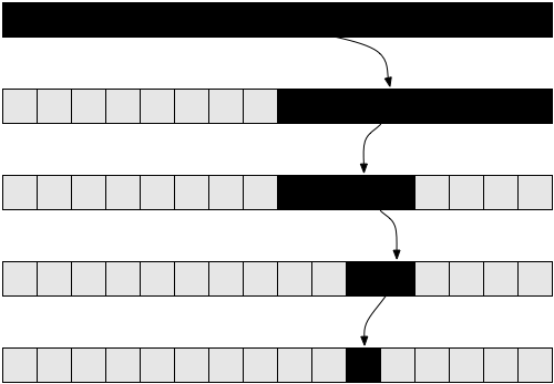
See Figure 6 to help you understand the way binary search operates.
If you're unsure that this method actually works, take a moment now to run it by hand in a simple example and convince yourself that it actually works.
Let us now attempt to analyze this algorithm. Again, we have a recursive algorithm in this case. Let's assume, for simplicity, that the array is always cut in exactly a half, ignoring just now the + 1 and - 1 part in the recursive call. By now you should be convinced that a little change such as ignoring + 1 and - 1 won't affect our complexity results. This is a fact that we would normally have to prove if we wanted to be prudent from a mathematical point of view, but practically it is intuitively obvious. Let's assume that our array has a size that is an exact power of 2, for simplicity. Again this assumption doesn't change the final results of our complexity that we will arrive at. The worst-case scenario for this problem would happen when the value we're looking for does not occur in our array at all. In that case, we'd start with an array of size n in the first call of the recursion, then get an array of size n / 2 in the next call. Then we'll get an array of size n / 4 in the next recursive call, followed by an array of size n / 8 and so forth. In general, our array is split in half in every call, until we reach 1. So, let's write the number of elements in our array for every call:
Notice that in the i-th iteration, our array has n / 2i elements. This is because in every iteration we're cutting our array into half, meaning we're dividing its number of elements by two. This translates to multiplying the denominator with a 2. If we do that i times, we get n / 2i. Now, this procedure continues and with every larger i we get a smaller number of elements until we reach the last iteration in which we have only 1 element left. If we wish to find i to see in what iteration this will take place, we have to solve the following equation:
1 = n / 2i
This will only be true when we have reached the final call to the binarySearch() function, not in the general case. So solving for i here will help us find in which iteration the recursion will finish. Multiplying both sides by 2i we get:
2i = n
Now, this equation should look familiar if you read the logarithms section above. Solving for i we have:
i = log( n )
This tells us that the number of iterations required to perform a binary search is log( n ) where n is the number of elements in the original array.
If you think about it, this makes some sense. For example, take n = 32, an array of 32 elements. How many times do we have to cut this in half to get only 1 element? We get: 32 → 16 → 8 → 4 → 2 → 1. We did this 5 times, which is the logarithm of 32. Therefore, the complexity of binary search is Θ( log( n ) ).
This last result allows us to compare binary search with linear search, our previous method. Clearly, as log( n ) is much smaller than n, it is reasonable to conclude that binary search is a much faster method to search within an array than linear search, so it may be advisable to keep our arrays sorted if we want to do many searches within them.
Rule of thumb: Improving the asymptotic running time of a program often tremendously increases its performance, much more than any smaller "technical" optimizations such as using a faster programming language.
Optimal sorting
Congratulations. You now know about analyzing the complexity of algorithms, asymptotic behavior of functions and big-O notation. You also know how to intuitively figure out that the complexity of an algorithm is O( 1 ), O( log( n ) ), O( n ), O( n2 ) and so forth. You know the symbols o, O, ω, Ω and Θ and what worst-case analysis means. If you've come this far, this tutorial has already served its purpose.
This final section is optional. It is a little more involved, so feel free to skip it if you feel overwhelmed by it. It will require you to focus and spend some moments working through the exercises. However, it will provide you with a very useful method in algorithm complexity analysis which can be very powerful, so it's certainly worth understanding.
We looked at a sorting implementation above called a selection sort. We mentioned that selection sort is not optimal. An optimal algorithm is an algorithm that solves a problem in the best possible way, meaning there are no better algorithms for this. This means that all other algorithms for solving the problem have a worse or equal complexity to that optimal algorithm. There may be many optimal algorithms for a problem that all share the same complexity. The sorting problem can be solved optimally in various ways. We can use the same idea as with binary search to sort quickly. This sorting method is called mergesort.
To perform a mergesort, we will first need to build a helper function that we will then use to do the actual sorting. We will make a merge function which takes two arrays that are both already sorted and merges them together into a big sorted array. This is easily done:
            def merge( A, B ):
                if empty( A ):
                    return B
                if empty( B ):
                    return A
                if A[ 0 ] < B[ 0 ]:
                    return concat( A[ 0 ], merge( A[ 1...A_n ], B ) )
                else:
                    return concat( B[ 0 ], merge( A, B[ 1...B_n ] ) )
The concat function takes an item, the "head", and an array, the "tail", and builds up and returns a new array which contains the given "head" item as the first thing in the new array and the given "tail" item as the rest of the elements in the array. For example, concat( 3, [ 4, 5, 6 ] ) returns [ 3, 4, 5, 6 ]. We use A_n and B_n to denote the sizes of arrays A and B respectively.
Exercise 8
Verify that the above function actually performs a merge. Rewrite it in your favourite programming language in an iterative way (using for loops) instead of using recursion.
Analyzing this algorithm reveals that it has a running time of Θ( n ), where n is the length of the resulting array (n = A_n + B_n).
Exercise 9
Verify that the running time of merge is Θ( n ).
Utilizing this function we can build a better sorting algorithm. The idea is the following: We split the array into two parts. We sort each of the two parts recursively, then we merge the two sorted arrays into one big array. In pseudocode:
        def mergeSort( A, n ):
            if n = 1:
                return A # it is already sorted
            middle = floor( n / 2 )
            leftHalf = A[ 1...middle ]
            rightHalf = A[ ( middle + 1 )...n ]
            return merge( mergeSort( leftHalf, middle ), mergeSort( rightHalf, n - middle ) )
This function is harder to understand than what we've gone through previously, so the following exercise may take you a few minutes.
Exercise 10
Verify the correctness of mergeSort. That is, check to see if mergeSort as defined above actually correctly sorts the array it is given. If you're having trouble understanding why it works, try it with a small example array and run it "by hand". When running this function by hand, make sure leftHalf and rightHalf are what you get if you cut the array approximately in the middle; it doesn't have to be exactly in the middle if the array has an odd number of elements (that's what floor above is used for).
As a final example, let us analyze the complexity of mergeSort. In every step of mergeSort, we're splitting the array into two halves of equal size, similarly to binarySearch. However, in this case, we maintain both halves throughout execution. We then apply the algorithm recursively in each half. After the recursion returns, we apply the merge operation on the result which takes Θ( n ) time.
So, we split the original array into two arrays of size n / 2 each. Then we merge those arrays, an operation that merges n elements and thus takes Θ( n ) time.
Take a look at Figure 7 to understand this recursion.
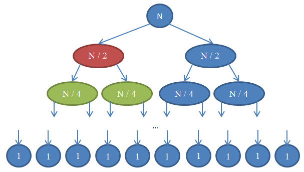
Let's see what's going on here. Each circle represents a call to the mergeSort function. The number written in the circle indicates the size of the array that is being sorted. The top blue circle is the original call to mergeSort, where we get to sort an array of size n. The arrows indicate recursive calls made between functions. The original call to mergeSort makes two calls to mergeSort on two arrays, each of size n / 2. This is indicated by the two arrows at the top. In turn, each of these calls makes two calls of its own to mergeSort two arrays of size n / 4 each, and so forth until we arrive at arrays of size 1. This diagram is called a recursion tree, because it illustrates how the recursion behaves and looks like a tree (the root is at the top and the leaves are at the bottom, so in reality it looks like an inversed tree).
Notice that at each row in the above diagram, the total number of elements is n. To see this, take a look at each row individually. The first row contains only one call to mergeSort with an array of size n, so the total number of elements is n. The second row has two calls to mergeSort each of size n / 2. But n / 2 + n / 2 = n and so again in this row the total number of elements is n. In the third row, we have 4 calls each of which is applied on an n / 4-sized array, yielding a total number of elements equal to n / 4 + n / 4 + n / 4 + n / 4 = 4n / 4 = n. So again we get n elements. Now notice that at each row in this diagram the caller will have to perform a merge operation on the elements returned by the callees. For example, the circle indicated with red color has to sort n / 2 elements. To do this, it splits the n / 2-sized array into two n / 4-sized arrays, calls mergeSort recursively to sort those (these calls are the circles indicated with green color), then merges them together. This merge operation requires to merge n / 2 elements. At each row in our tree, the total number of elements merged is n. In the row that we just explored, our function merges n / 2 elements and the function on its right (which is in blue color) also has to merge n / 2 elements of its own. That yields n elements in total that need to be merged for the row we're looking at.
By this argument, the complexity for each row is Θ( n ). We know that the number of rows in this diagram, also called the depth of the recursion tree, will be log( n ). The reasoning for this is exactly the same as the one we used when analyzing the complexity of binary search. We have log( n ) rows and each of them is Θ( n ), therefore the complexity of mergeSort is Θ( n * log( n ) ). This is much better than Θ( n2 ) which is what selection sort gave us (remember that log( n ) is much smaller than n, and so n * log( n ) is much smaller than n * n = n2). If this sounds complicated to you, don't worry: It's not easy the first time you see it. Revisit this section and reread about the arguments here after you implement mergesort in your favourite programming language and validate that it works.
As you saw in this last example, complexity analysis allows us to compare algorithms to see which one is better. Under these circumstances, we can now be pretty certain that merge sort will outperform selection sort for large arrays. This conclusion would be hard to draw if we didn't have the theoretical background of algorithm analysis that we developed. In practice, indeed sorting algorithms of running time Θ( n * log( n ) ) are used. For example, the Linux kernel uses a sorting algorithm called heapsort, which has the same running time as mergesort which we explored here, namely Θ( n log( n ) ) and so is optimal. Notice that we have not proven that these sorting algorithms are optimal. Doing this requires a slightly more involved mathematical argument, but rest assured that they can't get any better from a complexity point of view.
Having finished reading this tutorial, the intuition you developed for algorithm complexity analysis should be able to help you design faster programs and focus your optimization efforts on the things that really matter instead of the minor things that don't matter, letting you work more productively. In addition, the mathematical language and notation developed in this article such as big-O notation is helpful in communicating with other software engineers when you want to argue about the running time of algorithms, so hopefully you will be able to do that with your newly acquired knowledge.
About
This article is licensed under Creative Commons 3.0 Attribution. This means you can copy/paste it, share it, post it on your own website, change it, and generally do whatever you want with it, providing you mention my name. Although you don't have to, if you base your work on mine, I encourage you to publish your own writings under Creative Commons so that it's easier for others to share and collaborate as well. In a similar fashion, I have to attribute the work I used here. The nifty icons that you see on this page are the fugue icons. The beautiful striped pattern that you see in this design was created by Lea Verou. And, more importantly, the algorithms I know so that I was able to write this article were taught to me by my professors Nikos Papaspyrou and Dimitris Fotakis.
I'm currently a cryptography PhD candidate at the University of Athens. When I wrote this article I was an undergraduate Electrical and Computer Engineering undergraduate at the National Technical University of Athens mastering in software and a coach at the Greek Competition in Informatics. Industry-wise I've worked as a member of the engineering team that built deviantART, a social network for artists, at the security teams of Google and Twitter, and two start-ups, Zino and Kamibu where we did social networking and video game development respectively. Follow me on Twitter or on GitHub if you enjoyed this, or mail me if you want to get in touch. Many young programmers don't have a good knowledge of the English language. E-mail me if you want to translate this article into your own native language so that more people can read it.
Thanks for reading. I didn't get paid to write this article, so if you liked it, send me an e-mail to say hello. I enjoy receiving pictures of places around the world, so feel free to attach a picture of yourself in your city!
References
- Cormen, Leiserson, Rivest, Stein. Introduction to Algorithms, MIT Press.
- Dasgupta, Papadimitriou, Vazirani. Algorithms, McGraw-Hill Press.
- Fotakis. Course of Discrete Mathematics at the National Technical University of Athens.
- Fotakis. Course of Algorithms and Complexity at the National Technical University of Athens.

